Somebody asks how many workers the queue needs. The answers in the room are usually "ten feels right", "let's double it and see", or a number that was set eighteen months ago by a person who has since left. All three are guesses, and the arithmetic that replaces them takes about a minute.
At TRIBE the thing that made a hundred thousand users feel fast was moving expensive work off the request path into BullMQ and SQS, and once work is in a queue, "how many consumers" becomes the question that decides both your latency and your bill. This post is the maths behind that number: one law that always holds, one formula that usually holds, and the places where both stop describing your system.
The law that always holds
John Little proved it in 1961, and restated it fifty years later in Little's Law as Viewed on Its 50th Anniversary: "the average number of items in a queuing system, denoted L, equals the average arrival rate of items to the system, λ, multiplied by the average waiting time of an item in the system, W. Thus, L = λW."
What makes it useful is what it leaves out. It holds "independent of queue discipline" — first in first out, last in first out, priority classes, it makes no difference. It holds "under nonstationary conditions", so your traffic does not have to be steady. It says nothing about how arrivals are distributed or how long service takes. As Little puts it, the practical value is blunt: "If you know two of {L, λ, W}, you can quickly calculate the third."
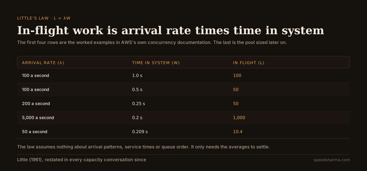
You have met this law already if you have read a cloud pricing page. AWS's Lambda concurrency documentation states it without naming it: "Concurrency = (average requests per second) (average request duration in seconds)". Their worked example is Little's law exactly: "Concurrency = (5,000 requests/second) (0.2 seconds/request) = 1,000". The same page makes the point that concurrency and requests per second are different quantities, which is precisely what W is doing in the formula.
The useful trick is running it backwards. You rarely measure W directly, but you can always see how many jobs are waiting and how fast they arrive. A queue holding 2,000 jobs that drains at 50 a second has jobs waiting 40 seconds. Nothing needs instrumenting; the backlog graph already told you your latency.
The number that is not the answer
Here is where the law gets misused. Take 50 jobs a second, each taking 200 ms. Multiply and you get 10. Ten what?
Ten is the offered load: the amount of work arriving per unit of time, measured in workers. It is the number of workers that would be busy every single second if jobs arrived in a perfectly even stream, spaced exactly 20 ms apart, each taking exactly 200 ms.
They do not arrive like that. Jobs arrive in clumps, some take longer than others, and a worker that finishes early cannot lend its spare moment to a worker that is busy. A pool of exactly ten in a world with any randomness in it is a pool that falls behind during every clump and never fully catches up, because it has no spare capacity to catch up with. Ten is a floor that you must stay above, not a size.
How far above depends on how long you are willing to let jobs wait, and that question has a formula of its own.
Why the last worker costs the most
For a pool of interchangeable workers taking jobs from one queue, with jobs arriving at random, the standard model is the M/M/c queue, and the quantity you want is the chance that an arriving job finds every worker busy. That is the Erlang C formula, stated here as
C(c, a) = (a^c / c!) · [ (1 − a/c) · Σ(i=0..c−1) a^i/i!  +  a^c/c! ]^(−1)

a = λ × service time   (offered load)
and once you have it, the average time a job spends queued is that probability divided by the pool's spare capacity:
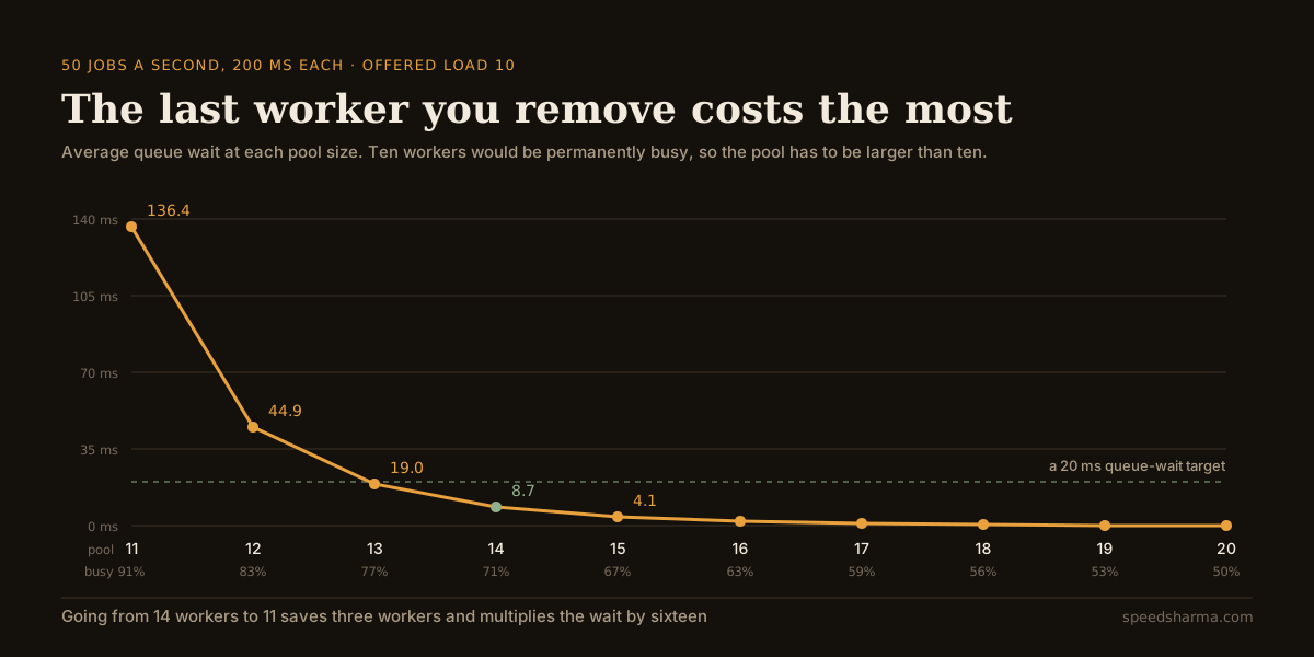
Wq = C(c, a) / (c/S − λ)Those two lines produce the whole table below. I checked them two ways before building anything on them: against a published worked example, where the formula reproduces the quoted answer of 0.702, and against a discrete-event simulation of the same queue, which agrees to within a few per cent.
| Pool size | Utilisation | Jobs that wait | Queue wait | Total latency |
|---|---|---|---|---|
| 11 workers | 90.9% | 68.2% | 136.4 ms | 336.4 ms |
| 12 workers | 83.3% | 44.9% | 44.9 ms | 244.9 ms |
| 13 workers | 76.9% | 28.5% | 19.0 ms | 219.0 ms |
| 14 workers | 71.4% | 17.4% | 8.7 ms | 208.7 ms |
| 16 workers | 62.5% | 5.7% | 1.9 ms | 201.9 ms |
Read the first column as money and the last as user experience. Going from 14 workers down to 11 saves three workers, a 21% saving, and multiplies the queue wait by more than fifteen. Going from 14 up to 16 costs two more workers and saves under 7 ms, which nobody will notice. The interesting decisions all live in a band a few workers wide.
The shape is not specific to these numbers. Queue wait scales roughly with 1/(1 − utilisation), so the cost of the next percentage point of utilisation rises as you approach the top. At 50% you are paying almost nothing for a burst; at 90% you are one slow dependency away from a backlog.
quick check
A queue receives 50 jobs a second and each job takes 200 ms of work. How many workers does it need?
50 × 0.2 = 10 is the offered load, meaning ten workers would be busy every second with nothing spare, so the queue would grow without bound. Eleven workers gives an average wait of 136 ms; fourteen gives 8.7 ms. The multiplication sets the floor; your latency target picks the number.
Size your own pool
Put in the arrival rate at your busiest minute rather than your daily average, and the time one job actually takes from pick-up to completion.
calculator · L = λW and Erlang C
How many workers does this queue need?
average queue wait at each pool size
Sizing uses two rules and takes whichever is larger: enough workers to keep average utilisation at or under your cap, and enough to hold the average queue wait under your target. Waiting time comes from the Erlang C formula for an M/M/c queue, which assumes jobs arrive at random and service times are exponentially distributed. Real service times are usually more variable, so treat every wait here as the best case for that pool size.
Two inputs deserve care. Arrival rate should come from your peak, because a pool sized for the daily mean is undersized for eight hours a day. Service time should be a high percentile rather than the median if your work is variable, because the formula assumes a distribution that is kinder than most real workloads.
Big pools beat small pools
One result from this maths is unintuitive enough to be worth stating on its own: larger pools can safely run at higher utilisation than smaller ones. Every row below sits at exactly 80% utilisation with the same 200 ms jobs. Only the pool size changes.
| Pool size | Arrival rate | Jobs that wait | Queue wait |
|---|---|---|---|
| 2 workers | 8 a second | 71.1% | 355.6 ms |
| 5 workers | 20 a second | 55.4% | 110.8 ms |
| 10 workers | 40 a second | 40.9% | 40.9 ms |
| 20 workers | 80 a second | 25.6% | 12.8 ms |
| 50 workers | 200 a second | 8.7% | 1.7 ms |
| 100 workers | 400 a second | 2.0% | 0.2 ms |
The reason is that a big pool has more ways to absorb a clump. In a pool of two, one slow job takes half your capacity. In a pool of fifty, it takes two per cent. Splitting one pool of twenty into four pools of five, with the work shared evenly between them, takes the average queue wait from 12.8 ms to 110.8 ms without changing a single machine.
This is why carving one queue into several specialised ones can make latency worse even though nothing else changed, and why the instinct to give each job type its own small pool needs a reason beyond tidiness.
The reason that does justify splitting is head-of-line blocking. If one job type takes thirty seconds and another takes fifty milliseconds, putting them in one queue means the fast ones wait behind the slow ones. Split by service time, not by feature area, and keep each pool as large as the split allows.
Where the model stops being true
Little's law is safe. The waiting-time formula is a model, and models have edges:
- Service times are not exponential. Real work has heavy tails: most jobs are quick and a few take a hundred times longer. Higher variability means longer waits than Erlang C predicts at the same utilisation. Treat the tool's output as a floor and measure the real thing.
- Arrivals are not always random. Traffic driven by cron jobs, retries or a partner's batch export arrives in bursts that no smooth model captures. A burst of a thousand jobs is a different problem from a rate of a thousand a second.
- Workers are not identical or independent. They share a database, a rate limit, a downstream API. Adding workers past the point where the shared resource saturates adds queueing, not throughput.
- The queue is not infinite. Every real queue has a memory limit or a retention window, and the interesting question past that point is which work you shed. That needs backpressure, and a plan for what happens when the backlog explodes.
- Jobs are not always safe to repeat. A worker pool that scales up under load will retry more, and retrying is only safe when the work is idempotent.
What I would actually do
- Measure λ at the peak minute, not the peak hour. Averaging over an hour hides the five minutes that hurt.
- Measure service time as a distribution. Take p50 and p95. Size with p95 if the spread is wide.
- Compute the offered load and refuse to run near it. λ × S is the floor. Aim for 70% to 80% average utilisation on a pool of a reasonable size.
- Alert on queue wait, not queue depth. Depth means nothing without the drain rate; wait is the number your users feel. Little's law converts one into the other for free.
- Autoscale on the same signal. Scaling on CPU misses the case where workers are blocked on a slow dependency, which is exactly when the queue grows.
- Split pools by service time. One pool for the fast work, one for the slow work, each as large as you can make it.
For request-serving systems the same arithmetic gives you thread and connection pool sizes, and the same warning applies: a pool sized exactly to the offered load has no capacity to recover from anything. The cost side of the same question, for AI workloads where each unit of work is priced, is in what an LLM costs per user, and the latency side of a real-time pipeline is in the voice agent latency budget.
questions people ask
What is Little's law?
L = λW. The average number of items in a system equals the average arrival rate multiplied by the average time each item spends there. It holds for any stable system regardless of arrival pattern, service time distribution or queue order.
How do I calculate how many workers I need?
Multiply the arrival rate by the service time to get the offered load, which is the number of workers that would be permanently busy. Then add capacity above that until the queue wait meets your target. For 50 jobs a second at 200 ms, the offered load is 10 and a realistic pool is 13 to 14.
What utilisation should a worker pool run at?
For most pools, 70% to 80% average utilisation is a reasonable target. Queue wait rises roughly with 1/(1 − utilisation), so 90% costs far more latency than it saves in machines. Larger pools can run closer to the top than small ones.
Does Little's law apply to database connection pools?
Yes. Connections in use equals query rate multiplied by query duration. It gives the floor for pool size, though the real limit is usually how much concurrency the database itself benefits from.
Why does latency explode as utilisation approaches 100%?
Because the spare capacity that lets a pool recover from a burst is exactly what utilisation consumes. The waiting time in a queueing model scales with 1/(1 − utilisation), so as utilisation approaches one, wait grows without bound.
Is Erlang C accurate for real workloads?
It is a useful lower bound rather than a prediction. It assumes random arrivals and exponential service times; real service times are usually more variable, which makes waits longer at the same utilisation.
The short version
Little's law, L = λW, is the one piece of queueing theory that always holds, and it takes a minute to apply. Multiply arrival rate by service time and you get the offered load: the workers that would be busy all the time. That is the floor.
The answer sits above the floor, and how far above is decided by how long jobs may wait. Queue wait rises roughly with 1/(1 − utilisation), so the last worker you remove costs far more than the first one you added. Size for 70% to 80%, alert on wait rather than depth, split pools by service time rather than by feature, and remember that the model flatters you: real work is more variable than the formula assumes.